Webmaster tools offered by Google and Bing, provide a source to obtain top searched keywords that search engines have returned pages from your website. Your web analytics is also an intelligence source to retrieve search terms that are driving traffic to your website. You might even want to pay a premium for access to competitive intelligence tools, i.e. ComScore, Hitwise in order to acquire the list of search terms that your competitors are ranking for.
You can easily identify certain individual keyword phrases and extend your keyword targeting around the popular searched keywords. If you are looking at competitors’ data, you can understand the keyword phrases that your competitors are targeting for, and thereby work on a strategy that will benefit your website.
Before you read on, check that your workstation is installed with Microsoft Excel. If you have a really long list of searched keywords, I suggest that Excel 2007 or later versions will be of a better choice. In Excel 2007, the maximum number of rows per worksheet increased to 1,048,576; while earlier Excel versions only have a maximum of 65,536 rows.
1. Working on Excel, place your list of searched keywords into one column.
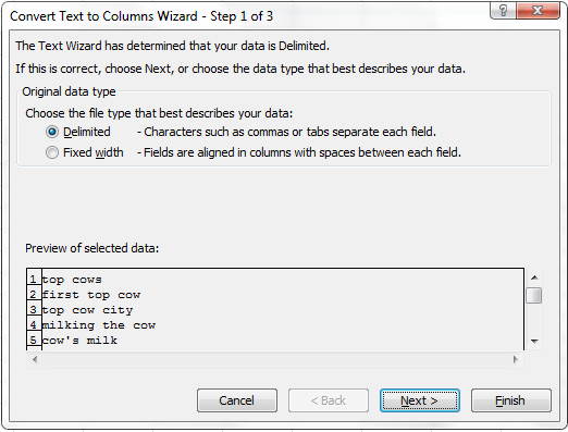
2. Select the column of keywords, click on “Text to Columns” function under the “Data” tab in Excel 2007.
In the wizard, choose the radio button: “delimiter” and click the Next button.
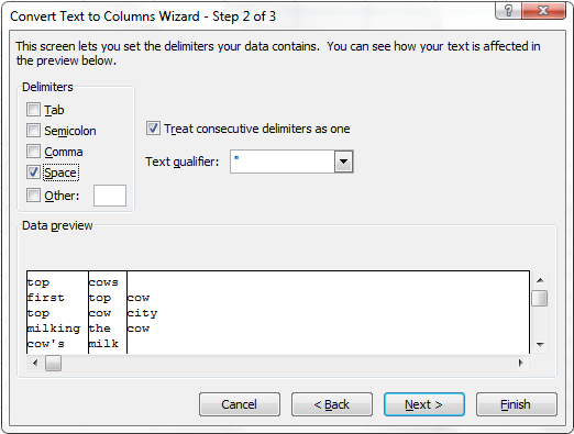
Select the checkbox: “Space” and click the Finish button.
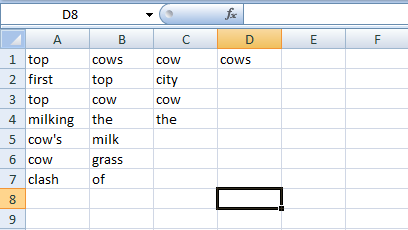
And your list of searched keywords are separated by spacing into the respective columns. If your search term has 4 words, the function will split the search term into 4 columns.
3. The searched keywords are broken down into individual search terms spanning across the columns unevenly with spaces between each rows. Select all the rows and columns. Click on the “Find & Select” > “Go To Special” function.
Select the radio button: “Blanks” and click the OK button. This will trigger Excel to automatically select all the blank cells.
Click on “Delete” > “Delete Cells” function, and select the radio button: “Shift cells up”. All the blank cells are deleted and the keywords are shifted to the top. If you performing this action on a large amount of keywords, Excel may require some processing time.
4. Shift all the keywords across the columns into a single column. This can be done in a manual manner by “cut & paste” in Excel. If you are an advanced Excel user, you can consider running a macro function:
Sub CopyToA()
Range(ActiveCell, ActiveCell.End(xlDown)).Cut Destination:=Range(“A1048576”).End(xlUp).Offset(1, 0)
End Sub
Select the column and run the macro function accordingly. This appends the selected column of keywords to the first column, Just a few clicks, all the keywords are transferred over to the first column.
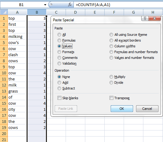
5. Use the COUNTIF function to count the number of occurrences that the individual keyword appears within the list.
=COUNTIF (A:A,A1)
Apply the function to each Excel row to perform the count for all keywords in the first column. Copy the results and “Paste Special” as “Values” to obtain the count.
6. Click on “Remove Duplicates” function under the “Data” tab. This will remove the duplicate values, leaving only each unique keyword with its respective occurrence count.
7. Sort the keywords with its occurrence count in a descending order. You can easily find out the individual top searched keywords.


